In recent months I have been investigating high dynamic range (HDR) support for the Linux desktop, and what needs to be done so that a user could, for example, watch a high dynamic range video.

The problem with HDR is not so much that there is no material out there covering it, but that there’s a huge amount of material can be rather confusing. I thought it best to add more material that is probably also confusing, but may help me think through HDR better. The following content is likely wrong as I have no background in colorimetry, the human visual system, or graphics generally. I’d love to hear what makes no sense.

In this post I’ll cover what HDR is and why we care about it. In the next post, I’ll cover the work in specific projects that has been done to support it and what is left to be done.

Background

Before attempting to understand dynamic range, I found it helpful to understand the basics of electromagnetic radiation (light) and how the human visual system (eyes) interact with light so that we can produce graphics for human consumption. With an understanding of how to do that, we can complete our ultimate goal of tricking the human visual system into seeing extremely realistic images of cats even if there are no cats around.

Light

Light can be described as a wave with an amplitude and frequency/wavelength or a particle (photon) with a frequency/wavelength. Human eyes detect a very small frequency range of electromagnetic radiation. More particles is equivalent to a higher amplitude wave. The range of wavelengths eyes typically see is approximately 380 nanometers to 750 nanometers.

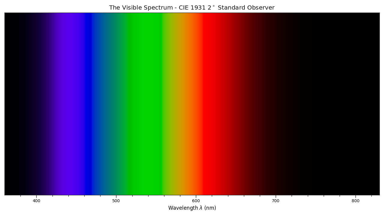
Humans detect wavelength of light as colors, with blue in the 450-490nm range, green in 525-560nm range, and red in the 630-700nm range.

More photons of a given wavelength are perceived by humans as a brighter light of the color associated with the wavelength.

Luminance

Luminance is the measure of the amount of light in the visibile spectrum that passes through an area. The SI unit is candela per square meter (cd/m²). This is often also referred to as a “nit”, presumably because cd/m² is somewhat laborious to type out.

The human eye can detect a luminance range from about 0.000001 cd/m² to around 100,000,000 cd/m². We can readily go out into the world and experience this entire range, too. For example, the luminance of the sun’s disk at noon is around 1,600,000,000 cd/m². This is much higher than the human eye can safely experience; do not go stare at the sun.

One important detail is that the human perception of luminance is roughly logarithmic. You might already be familiar with this as decibels are used to describe sound levels. The fact that human sensitivity to luminance is non-linear becomes very important later when we need to compress data.

Human Visual System

The eye is composed of two general types of cells. The rod cells which are very sensitive and can detect very low amplitude (brightness) light waves, but don’t differentiate between wavelengths (color) well.

The cone cells, by contrast, come in several flavors where each flavor is sensitive to a different wavelength. Many humans have three flavors, imaginatively referred to as S, M, and L. S detects “short” wavelengths (blue), M detects “medium” wavelengths (green), and L detects “long” wavelengths (red).

Different colors are produced by stimulating these cone cells in with different ratios of wavelengths.

One thing to keep in mind, as it adds a minor complication to calculating luminance, is that not all the cone cells are equally sensitive. If you were to take a blue light, a green light, and a red light that all emit the same number of photons, the green light would appear the brightest by far. The luminance, therefore, depends on the wavelength of the light.

While the human visual system is capable of detecting a very large range of luminance levels, it cannot do so all at once. If you’re outside on a sunny day and walk into a dark room, it takes some time for your eyes to adjust to the new luminance levels.

Color Spaces

When discussing displays and their capabilities you will hear about color spaces and perhaps see a diagram like this:

There’s a lot going on in this diagram and it is rather confusing (to me, anyway), so it’s worth covering the basics. There are some good blog posts with much more detail.

You’ll notice the outside curve of this color blob has numbers marked along them. These are light wavelengths, and the outer curve is the color we see for that pure wavelength. On the bottom edge there are no wavelengths. This is because those colors are what we see when the long cones and the short cones both sense light. All the colors not on the edge of the curve are created by blending together multiple wavelengths of light.

Often, you’ll hear people talk about the “temperature” of light. This is in reference to how as objects heat up they begin emitting light in the visible spectrum. The curve starting on the red side, passing through the center, and continuing toward blue shows the mapping of temperature to colors.

If we pick three points on this plane and form a triangle, we can create any color enclosed by the triangle by adding various ratios of those three colors together. These points have coordinates in this two-dimensional space, and we can describe the triangle by providing those coordinates. Using this approach, we can describe the colors a display can create by specifying three pairs of coordinates. This is the “color space”.

If you’re using GNOME, you can see a diagram of your display’s color gamut by going to the “Color” settings section, selecting the color profile, and clicking view details:

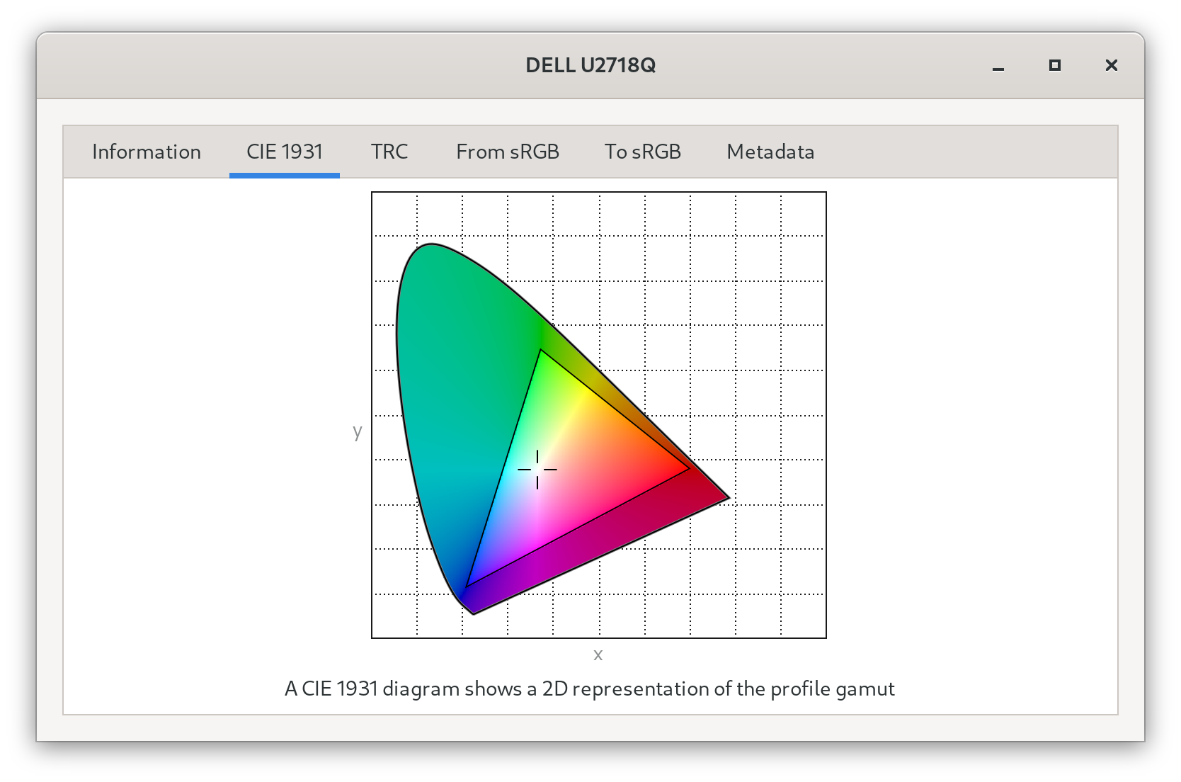
Note that these diagrams do not include the luminance. Doing so creates a third dimension and can be used to visualize a “color volume”.

Displays

There are several ways to display images for human consumption. One way is to reflect light off a surface that absorbs some frequencies of light and reflect the rest into the eye (paintings, books, e-ink, etc). The other way is to produce light to shine into the eye, such as the liquid crystal or organic LED screen you’re probably looking at right now.

There’s a few challenges with producing the light directly. The first is that we need to produce a range of light frequencies to cover the visible spectrum of human vision. As humans usually have three types of frequency-sensing cells, we don’t necessarily need to produce every single frequency in the visible spectrum. Instead, we can pick three frequencies that align with where the cone cells are sensitive and by adjusting the ratio of these three produce light that contains all information the human eye uses and none of the information it cannot detect.

This is why a display pixel is typically made up of blueish, greenish, and reddish components. Since this isn’t a perfect world, displays don’t tend to be capable of producing a single frequency. The frequency range of these components impact how the three overlapping cone sensitivities can be stimulated and therefore determine the range of colors the display is capable of producing. This range is referred to as the display’s “color gamut”. The color gamut can vary quite a bit from display to display, so we need to account for this when we encode images. We also need to handle cases where the display cannot produce the color we wish to show. We could not, for example, accurately display an image of a laser emitting pure 525nm light unless the green sub-pixel happened to also emit pure 525nm light. This is called “gamut mapping” as we map one color gamut to another color gamut.

The second issue is that if we want to perfectly replicate the real world, we would need to be able to emit light in the range of 0.000001-1,600,000,000 cd/m². However, as we’ve already established, the sun is not safe to look at so it would be best to not faithfully reproduce it on a display. Even if we restrict ourselves to the 0.000001-100,000,000 cd/m² range, the power requirements and heat produced would be astronomical. We have to attempt to represent the world using a smaller luminance range than we actually experience. In other words, we have to compress the luminance range of our world to fit the luminance range of the display. This process is often referred to as “tone-mapping”.

Dynamic Range

Dynamic range is the ratio between the smallest value and largest value. When used in reference to displays, the value is luminance.

The lowest luminance level is determined by how much ambient light is reflecting off the surface of the display (e.g. are you sitting in a dark room, outside on a sunny day, etc), how much of the backlight (if there is one) leaks through the display panel, and so on.

The highest luminance level is determined by the light source of the display. This depends on the type of display, power usage requirements, user preferences, on the ambient temperature (emitting visible light also emits heat, and excessive heat can damage the display components), and perhaps other factors I am not aware of.

As both these values depend on environmental factors the dynamic range of a display can change from moment to moment, which is something we may wish to account for when compressing the luminance range of the world to fit the particular display.

So what is a high dynamic range display? In short, a display that is simultaneously capable of lower luminance levels and higher luminance levels than previous “standard dynamic range” displays. What these levels are exactly can be hand-wavy, but VESA provides some clear specifications.

This higher dynamic range ultimately means the way in which we compress the luminance range (tone-map) needs to change.

Light from Scene to Display

Now that we know the pieces of the puzzle, we can examine how an image ends up on our displays. In this section, we’ll cover the journey of an image from its creation to its display. Perhaps the most self-contained example is a modern video game. This allows us to dodge the added complication of camera sensors, but the process for real-world image capture is similar.

Scene-referred Lighting

Video games typically model a world complete with realistic lighting. When they do this, they need to work with “real world” luminance levels. For example, the sun that lights the scene may be modeled to be seen as 1.6 billion nits. Working with real world luminance that cannot be directly displayed is often called “scene-referred” luminance. We have to transform the scene-referred luminance levels to something we can display (“display-referred” luminance) by compressing or shifting the luminance values to a displayable range.

You might think it’s best to leave content in scene-referred lighting levels until the last possible moment (when the display is setting the value for each pixel), and that would indeed make some things simpler. However, it makes some things more difficult, like attempting to blend the scene-referred image with an image that is already display-referred. When doing operations like that, we need every part to be in the same frame of reference, either scene-referred or display-referred.

There’s a more difficult problem with keeping all content scene-referred, though. Representing numbers accurately in the 0.000001-1,600,000,000 cd/m² range requires a lot of bits, and we’re about to have a serious bit budget imposed on us. We have to transport the image data from the host graphics processing unit to the display. While both HDMI and DisplayPort have rather enormous bandwidth, the image resolution is also quite large. If we used a 32 bit floating point number for each red, green, and blue (RGB) component of a pixel on a display with 3840 x 2160 (4K) pixels, it would require 32 x 3 x 3840 x 2160 bits per frame, or 760 Mbits per frame. At a modest 60 frames per second, that’s 44.5 Gbits. DisplayPort 1.4 provides 25.9 Gbits and HDMI 2.0 give us 14.4 Gbits.

Fortunately for us, as long as we ensure the way we encode luminance levels matches up with the way the human eye detects luminance levels, we can save a lot of bits. In fact, for the “standard” dynamic range, we can manage with only 8 bits (256 luminance levels) per color (24 bits total for RGB).

Tone-mapping

In order to convert scene-referred, real world luminance to a range for our target display, we need to:

1. Have an algorithm for mapping one luminance value to another. Input values have a range [0,∞) and the output values need to cover the range of our target display.

2. Know the capability of our target display.

For now we’ll focus on #1, although #2 is important and, unfortunately, somewhat tricky.

There are many different approaches to tone-mapping and results can be subjective. This is not a post about tone-mapping (there are many multi-hundred page publications on the subject), we’ll just go over a couple examples to get the idea.

An extremely silly, but technically valid tone-mapping algorithm would be f(x) = 1, where x is the input luminance. This maps any input luminance level to 1.

A more useful approach might be the function f(x) = xⁿ/(xⁿ + sⁿ) where x is the input luminance, n is a parameter changes the slope of the mapping curve, and s shifts the curve on the horizontal axis. As a somewhat random example, with n = 3 and s = 10:

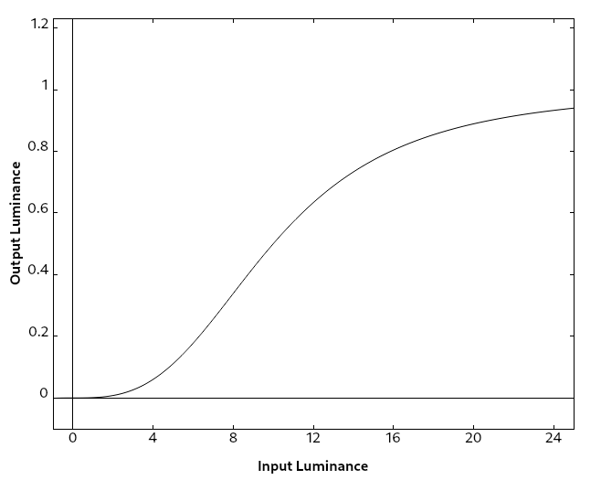
This sigmoid function gently approaches the minimum and maximum values of 0 and 1. We can then map the [0, 1] range to the display luminance range.

There are many articles and papers out there dedicated to tone mapping. There’s a chapter on the topic in “The high dynamic range imaging pipeline” by Gabriel Eilertsen, for example, which include a number of sample images and a much more thorough examination of the process than this blog post.

This process is occasionally referred to as an “opti-optical transfer function” or “OOTF” as it maps optical (luminance) values to different optical values. Note that it is also possible to tone-map luminance values that are encoded for storage or transportation, so-called “electronic” values, which you might see referred to as electro-electronic transfer functions or “EETF”

Encoding

Once we’ve tone-mapped our content to use the display’s luminance range, we need to send the content off to the display so that we can see it. As the section on scene-referred light mentioned, we have a limited amount of bandwidth, and any increase or decrease in bits used per pixel impacts how many bits are required for a frame, and thus how many frames we can send to the display every second. The key is to use as few bits as we can get away with.

The method used to encode luminance levels is called the “transfer function”, “opto-electronic transfer function”, or “OETF”. These are functions that approximate the human’s sensitivity to luminance levels.

Since the display needs to decode the encoded data we send it back to linear luminance values, we need functions that can be easily “undone” with an inverse function. The property we’re looking for in our encoding and decoding functions is g(f(x)) = x. This is called the “inverse transfer function”, “electro-optical transfer function”, or “EOTF” since it converts the “on-the-wire” values back to optical values.

Note that the terminology and definitions of these transfer functions can be confusing and vague. Some people appear to use OETF to mean both a tone-mapping operation and a transfer to electronic values.

Encoding SDR

The “standard dynamic range” is not particularly standard, but usually tops out around 300 nits. Typically, 8 bits per RGB component is used. 8 bits allow us to express 256 luminance levels per component.

The Naïve Approach

One method to encoding would be to evenly spread each level across the luminance range. What would this look like? In our thought experiment, we’ll assume the monitor’s minimum luminance is 0.5 nits, and its maximum luminance is 200 nits. This gives us a range of 199.5 nits. Equally distributed, each step increases the luminance by about 0.78 nits.

Sending [0, 0, 0] for red, green, and blue results in the minimum luminance of 0.5 nits. Adding a step [1, 1, 1] would result in 1.28 nits.

Sending [254, 254, 254] results in 198.44 nits, and sending [255, 255, 255] results in 200 nits.

The problem with this approach is that with lower luminance values, each step is above what the human eye differentiate, its just-noticeable difference. At higher luminance levels, each step is so far below the just-noticeable difference that it would require many steps for a human to notice any difference at all. It results in clearly visible bands in the lower luminance areas of the image we display and completely undetectable detail in the higher luminance areas of the image. We could resolve this by adding more bits (and therefore more levels), but we can’t afford to do that without giving up resolution and framerate.

Instead, we want to take these wasted levels at high luminances and use them in lower luminances.

Gamma

The “gamma” transfer function has a long and interesting history and is part of the sRGB standard. The sRGB version is actually a piecewise function which uses the gamma function for all but the very lowest luminance levels, but we can ignore that complication here.

The basic function is in the form f(x) = Axᵞ. In sRGB, A = 1.055 and 𝛾 = 1/2.4. The inverse function used to decode the luminance is A = 1/1.055 and 𝛾 = 2.4

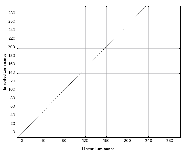
The encoding curve looks like this:

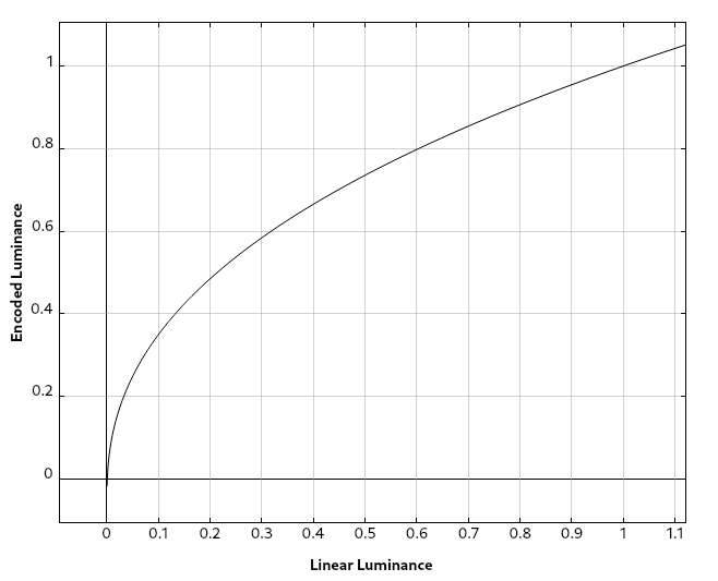
In this graph, we map the linear, display-referred luminance values into the range [0, 1]. These input luminances are mapped to an encoded value also in the range [0, 1]. We can see from the graph above that the lower third of the linear luminance levels get mapped on the lower two thirds of our encoding range.

We can convert the output to integer values between 0 and 255 by multiplying the encoded luminance value by 255 and rounding:

Now, instead of wasting many of our precious bits on luminance steps on the high end that no one can see, we’re spending most of them on low luminance levels.

This is a pretty good approach when we have 256 steps (8 bits) per component and luminance range of a few hundred nits, but the further we stretch the range of nits, the bigger our steps have to be, and eventually we’ll cross a point where some steps are about the just-noticeable difference line.

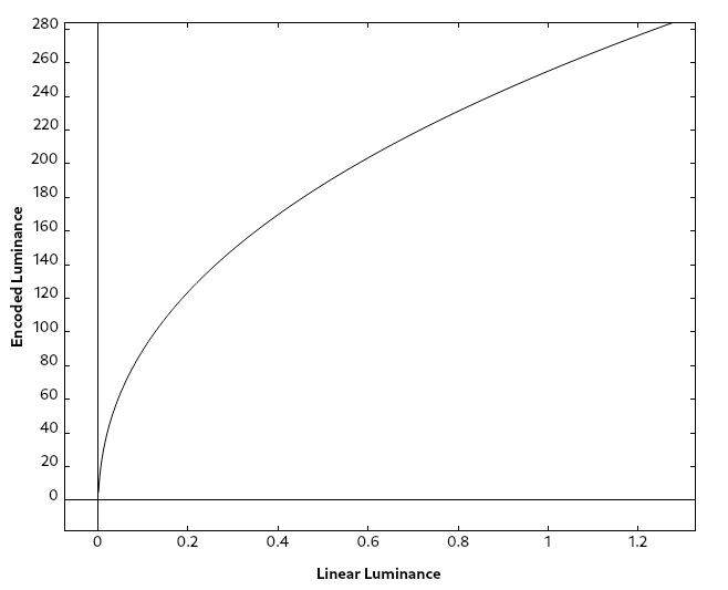
We can fix this by increasing the number of bits used. What happens if we move to 10 or even 12 bits? At 12 bits per component, we have 4096 steps.

At first glance this seems fine, but what if we adjust the graph to display actual nit values for the linear light? Here’s the same graph with linear light using a range of 0-1000 nits.

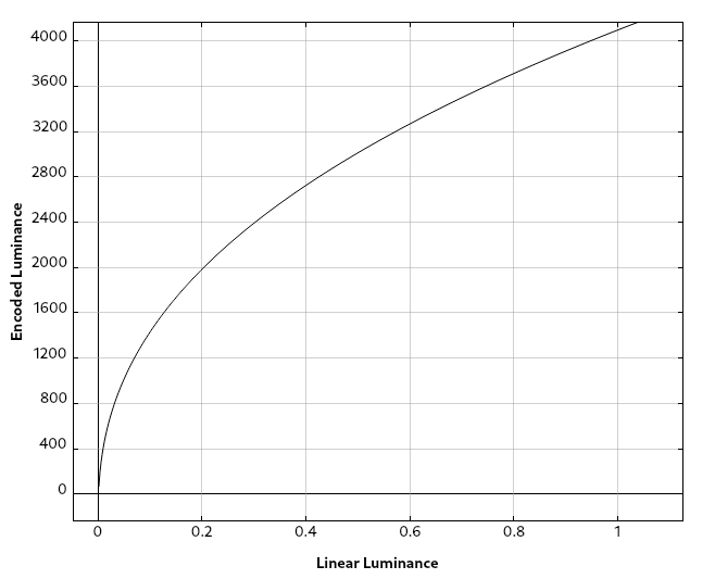
We can see that fewer than half our steps, or approximately 2000, land in the luminance ranges we use today for standard dynamic range displays. Once again, we’re allocating too many steps to the very high luminance levels where the human eye becomes less and less sensitive. This is even worse as the luminance range increases:

Thus, for displays with a higher dynamic range, we may want to adjust the transfer function to get the most value out of each bit we spend.

Encoding Higher Dynamic Ranges

As we saw when examining the gamma transfer function, it works reasonably well for low luminance ranges, but as the range increases it starts to be sub-optimal.

There are two major approaches for higher dynamic range encoding. Both have advantages and disadvantages, and displays can support either or both. If you’re curious if your displays are capable of using either of these approaches, you can check by installing edid-decode and running:

find /sys/devices -name edid -exec edid-decode {} \;

Look for a “HDR Static Metadata Data Block” and see what is included in the electro-optical transfer function list. This section will likely not be present if your display doesn’t support HDR.

The Perceptual Quantizer

The Perceptual Quantizer (PQ) transfer function, sometimes referred to by the much less cool name “SMPTE ST 2084”, defines a new curve to use for encoding. It is unlike the gamma transfer function in that it is defined to cover a well-defined luminance range, rather than just being fit to whatever the display happens to be capable of. The luminance range the curve is defined to cover is 0.0001-10,000 cd/m².

This is a useful concept when encoding the content as we can now express physical quantities in addition to “more/less luminance”. It gives the decoding side a frame of reference if it needs to further tone-map the content.

The curve looks like:

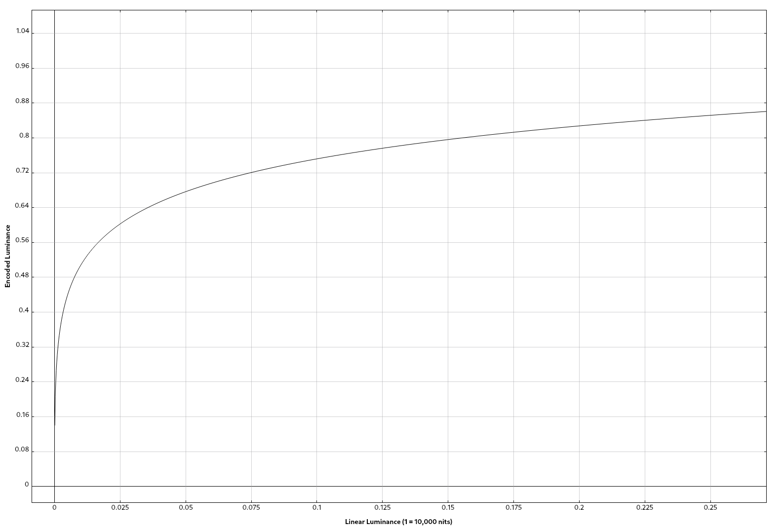
This graph is only part of the curve, and you can see the slope is so extreme it doesn’t render very well. It packs a vast majority of the code points into the lower luminance range where the eye is most discerning. Currently, it’s common to use this curve with 10 bits per component.

The function that describes this curve is more complicated than the gamma curve so I won’t attempt to render it poorly here. The curious can consult the Wikipedia page linked above.

The perceptual quantizer transfer function can be paired with metadata describing the image or images it is used to encode. This metadata is usually the primary colors of the display used to create the content as well as luminance statistics like the image’s minimum, maximum, and average luminance. This metadata allows consumers of the content to perform better tone-mapping and gamut-mapping since it describes the exact color volume of the content.

The PQ curve supports encoding luminance up to 10,000 nits, but there are no consumers displays capable of that. Even professional displays built for movie-making are well short of that, currently around 4,000 nits. This is still much higher than current consumer displays, so the metadata can be used to tone-map and gamut-map the content from the capabilities of fancy display the film studio used to the capabilities of the individual display. In the future, when consumer monitors become more capable, the same films will look better as they require less tone-mapping and the original intent can be more accurately rendered.

The Hybrid Log-Gamma

As the name suggests, the second approach for higher dynamic range encoding is to use a hybrid of the gamma function and a log function. The hybrid log-gamma (HLG) curve is designed with backwards-compatibility in mind.

HLG uses a piecewise function defined as follows when the input luminance has been normalized to a range of 0-1:

• When the input luminance L is between 0 and 1/12: sqrt(3) * L^0.5 (this is our old friend the gamma function f(x) = Axᵞ, with A = 1.732 and 𝛾 = 1/2)

• When input luminance L is between 1/12 and 1: a * ln(12L - b) + c where a = 0.17883277, b = 1 - 4a, and c = 0.55991073.

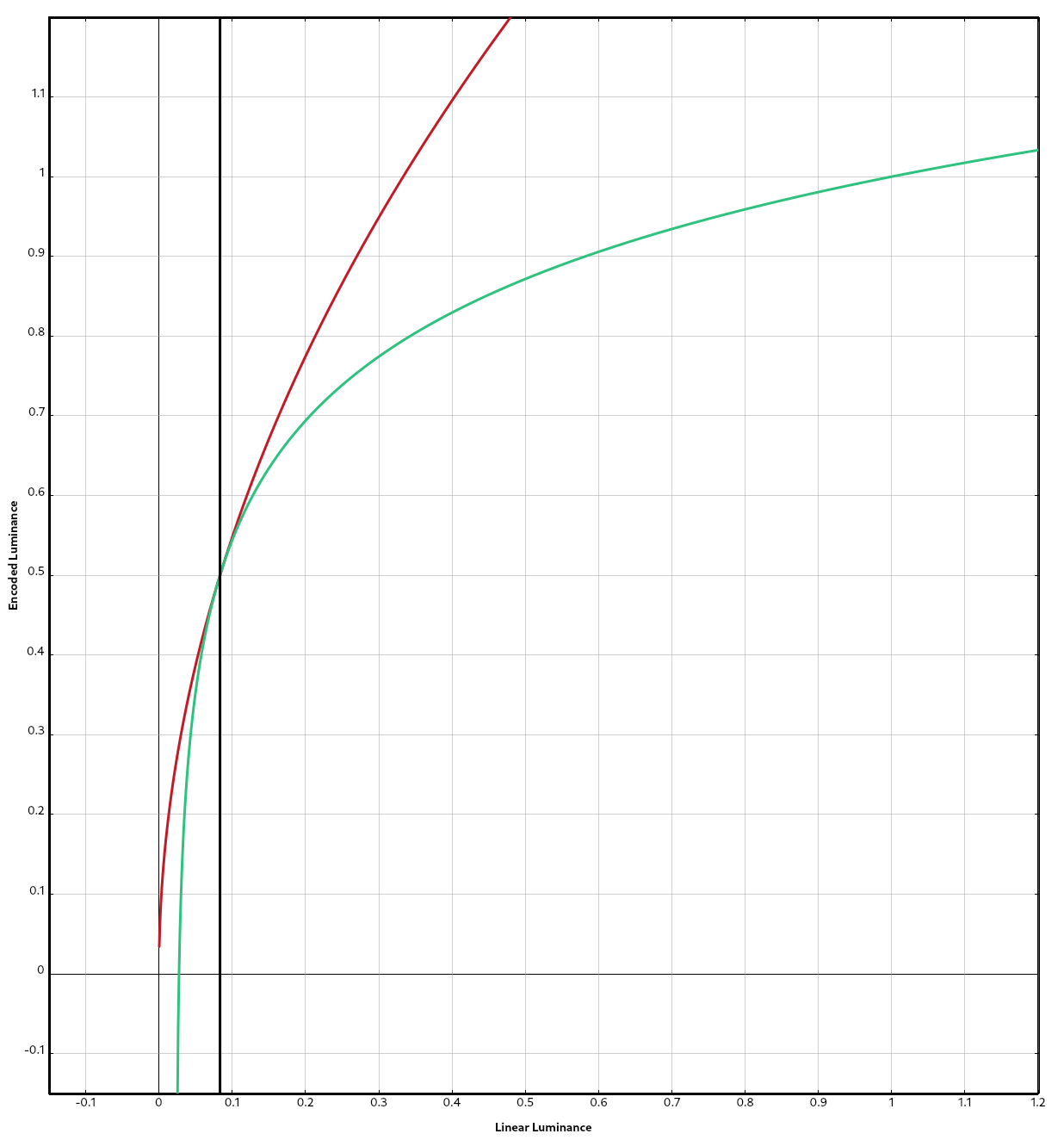
In the above graph, the red curve is the gamma curve, the green curve is the log curve, and the vertical line is the point where the gamma curve stops being used in favor of the log curve when encoding.

As this encoding scheme is defined in terms of relative luminance like the gamma transfer function, there is no metadata for tone-mapping.

Transmission and Display

Once we’ve encoded the image with a transfer function the display supports, the bits are sent to the display via HDMI or DisplayPort. At this point, what happens next is up to whatever is on the other end of the cable. I have not pulled apart a display and learned what secrets it holds, but we can make some reasonable guesses without destroying anything:

1. If metadata is provided (PQ-encoded images only), the display examines it and determines of any tone-mapping is required due to the content exceeding its capabilities. If it’s not provided, it likely assumes the content spans the entire range defined by PQ.

2. If the display includes light sensors to detect ambient light levels, it might decide to tone-map the content, even if it’s capable of displaying all luminance levels encoded.

3. Displays tend to include configuration to alter the color and brightness. It will take these into account when deciding if/how to tone-map or gamut-map the content we gave it.

4. Some gamut-mapping and tone-mapping will occur in the display depending on all the above variables, at which point it will emit some light.

Now, that’s a very high-level overview of the process, but we can map these high-level steps to portions of the Linux desktop and discuss what needs to change in order for us to support HDR.

Summary

Now that we understand (in theory) HDR, it’s worth asking what all this is good for.

If, as part of your movie-watching experience, you want an eye-wateringly bright sunset where you can still make out the blades of grass in the shadow of a rock this is an important feature. The more cinematic video games could look even better. These are the most obvious applications, and where many users will encounter HDR, but it’s not necessarily limited to entertainment. HDR is all about transmitting and displaying more information, so any process that involves visualization could benefit from more luminance levels.

As we’ll see in the next post, however, there is a good bit of work left to be done before you can, for example, enjoy an HDR film in GNOME’s Videos application.